
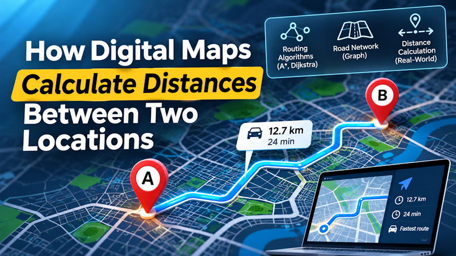
Digital maps make it surprisingly easy to find the distance between two places. Enter a starting point, choose a destination, and within seconds, a route appears with distance measurements and an estimated travel time.
But what actually happens between entering those two locations and receiving the final result?
Behind this seemingly simple process are several technologies working together. Digital mapping systems identify geographical coordinates, calculate distances across the Earth's surface, analyze connected road networks, and generate routes based on the selected mode of transportation.
Understanding these processes reveals why the distance between two cities can be different depending on whether you measure it geographically or calculate an actual driving, walking, or cycling route.
Let's explore how digital maps perform these calculations and what makes modern distance measurement possible.
1. Every Distance Calculation Starts With Geographic Coordinates
A digital map cannot calculate a meaningful distance from a place name alone. It first needs to identify the precise geographical position of the starting point and destination.
This is where latitude and longitude become important.
Latitude identifies how far north or south a location is from the Equator. Its values range from 0° at the Equator to 90° north or south.
Longitude identifies how far east or west a location is from the Prime Meridian, with values extending up to 180° in either direction.
Together, these coordinates represent a specific position on Earth's surface.
For example, a mapping application receiving a request to calculate the distance between Paris and Berlin must first identify the geographical coordinates associated with both cities.
It can then use those coordinates as inputs for distance calculations and route searches.
The same principle applies when searching for airports, landmarks, streets, or individual points on an interactive map.
How does a map identify the coordinates of a place?
Most digital mapping systems use a process called geocoding.
Geocoding converts a human-readable location, such as a city name, street address, or landmark, into geographical coordinates.
For example:
- Input: Eiffel Tower, Paris, France.
- Latitude: Approximately 48.8584° N.
- Longitude: Approximately 2.2945° E.
The mapping system can now work with numerical coordinates instead of the original text.
The reverse process is known as reverse geocoding. It takes geographical coordinates and attempts to identify the corresponding street address, locality, or named place.
Accurate location identification is important because even a small difference in the selected starting or ending coordinates can affect the final distance.
2. How Digital Maps Calculate Straight-Line Distance
Once both locations have been converted into coordinates, a mapping system can calculate the geographical distance separating them.
One commonly used mathematical method is the Haversine formula.
Unlike ordinary distance calculations on a flat surface, this formula accounts for the Earth's curvature by estimating the shortest distance along a spherical surface between two geographical points.
This measurement is commonly called great-circle distance or straight-line distance.
Understanding the Haversine formula
The Haversine formula uses four coordinate values:
- Latitude of the starting point.
- Longitude of the starting point.
- Latitude of the destination.
- Longitude of the destination.
It converts the differences between these coordinates into angular measurements and uses trigonometric functions to estimate the distance.
The formula can be expressed as:
a = sin²(Δφ/2) + cos(φ₁) × cos(φ₂) × sin²(Δλ/2)
c = 2 × atan2(√a, √(1 − a))
d = R × c
Where:
- φ₁ and φ₂ represent the latitudes of the two locations in radians.
- λ₁ and λ₂ represent their longitudes in radians.
- Δφ represents the difference in latitude.
- Δλ represents the difference in longitude.
- R represents the assumed radius of the Earth.
- d represents the calculated geographical distance.
For many everyday applications, the result provides a useful approximation of the distance between two geographical coordinates.
However, the Haversine formula does not consider roads, bridges, buildings, pedestrian paths, or other obstacles.
It measures geographical separation, not the distance someone would actually travel.
Why do developers use the Haversine formula?
The formula is useful because it is relatively straightforward to implement and works with coordinate pairs.
It can be applied to applications involving:
- Nearby location searches.
- Geographical data analysis.
- Distance-based filtering.
- Fitness and activity tracking.
- Basic navigation calculations.
- Location-based services.
Developers working with Google Maps can also use its Geometry library to calculate the spherical distance between two geographical points.
For a practical JavaScript implementation, see this tutorial on calculating the distance between two geographic coordinates, which demonstrates both the Google Maps Geometry method and the Haversine approach.
3. Why Straight-Line Distance Is Different From Road Distance
Knowing the geographical distance between two places does not necessarily tell you how far someone needs to travel.
Imagine two towns separated by a river.
Their geographical coordinates might indicate that they are only 15 kilometers apart. However, if the nearest bridge is located 20 kilometers away, the actual driving distance could be considerably longer.
This difference exists because roads and transportation networks do not follow perfectly straight lines.
They must accommodate geographical features, buildings, property boundaries, traffic regulations, and infrastructure.
A mapping system therefore needs a different approach when calculating an actual travel route.
Instead of measuring the direct separation between two coordinates, it must identify a connected path through a network of roads or accessible pathways.
This is where route calculation becomes important.
4. How Route Calculation Algorithms Find the Best Path
Digital maps generally represent transportation networks as interconnected graphs.
In graph theory, a graph consists of nodes and edges.
For a road network:
- Nodes represent intersections, junctions, or other relevant geographical points.
- Edges represent the roads or pathways connecting those points.
Each edge can contain additional information, including distance, permitted travel modes, speed restrictions, and other routing characteristics.
When someone requests directions between two locations, the routing system identifies suitable starting and ending nodes and searches for a connected path between them.
Dijkstra's algorithm
One established method for finding the shortest path through a network is Dijkstra's algorithm.
It explores connected nodes while maintaining the lowest known accumulated cost from the starting point.
For distance-based routing, that cost can represent the total length of the selected road segments.
The algorithm continues exploring the network until it identifies the shortest available path to the destination.
Dijkstra's algorithm is useful for understanding how shortest-path calculations work, although production mapping systems often use more advanced optimizations.
A* search algorithm
A* is another widely used pathfinding algorithm.
It combines the cost already accumulated along a route with a heuristic estimate of the remaining distance to the destination.
This helps guide the search toward the destination instead of exploring every possible connection equally.
For geographical routing, a straight-line distance estimate can serve as a heuristic when designed to remain admissible for the selected cost function.
A* can therefore explore large networks more efficiently than an uninformed search in many situations.
Shortest route versus fastest route
An important distinction is that the shortest route is not always the fastest.
Consider two possible journeys:
- Route A covers 25 kilometers through local roads.
- Route B covers 32 kilometers using a highway.
Although Route A is shorter, Route B might take less time because it allows higher average speeds and fewer stops.
Mapping systems can optimize routes using different objectives, such as distance, estimated travel time, or other transportation-specific costs.
The result depends on what the routing engine is designed to prioritize.
5. Why Driving, Walking, and Cycling Routes Produce Different Distances
A single pair of geographical coordinates can produce several different travel distances.
The reason is that not every transportation mode has access to the same network.
A car generally follows roads where motor vehicles are permitted. A pedestrian might use sidewalks, footpaths, pedestrian crossings, and walking trails.
Cyclists may have access to dedicated bicycle lanes, shared paths, and roads that are unsuitable or restricted for other transportation modes.
Modern routing systems account for these differences through transportation-specific network data and routing profiles.
Driving routes
Driving calculations generally use roads accessible to motor vehicles.
Depending on the routing configuration, the system may consider one-way restrictions, road classifications, turn restrictions, and other vehicle-related rules.
Walking routes
Walking calculations can include pedestrian pathways, sidewalks, crossings, and other accessible connections.
A pedestrian route might therefore be shorter than the equivalent driving route.
Cycling routes
Cycling calculations may prioritize bicycle-accessible roads, dedicated cycling infrastructure, and permitted shared pathways.
The route can differ considerably from both driving and walking options.
This is why a useful travel distance calculator should distinguish between transportation modes rather than assuming that every journey follows the same road network.
6. How Digital Maps Turn Calculated Routes Into Interactive Maps
Calculating a distance is only one part of the mapping process.
Users also need to see where the route goes.
Interactive digital maps combine geographical data, map tiles, and location coordinates to display roads, landmarks, boundaries, and other features.
When a route is calculated, the routing service typically returns a sequence of geographical points describing the path between the selected locations.
The mapping application then uses these points to draw a line or route overlay on the map.
This allows users to visualize the journey instead of relying exclusively on a numerical result.
The role of mapping libraries
Developers commonly use mapping libraries to build interactive map interfaces.
For example, Leaflet is an open-source JavaScript library that allows developers to display maps, add markers, draw geographical shapes, and interact with location data.
However, a mapping library and a routing engine perform different jobs.
A mapping library displays geographical information, while a routing engine calculates paths through a transportation network.
They can work together, but displaying a map does not automatically provide route calculations.
This distinction is important when developing location-based applications because both components need appropriate data sources.
7. How Digital Maps Estimate Travel Time
After calculating a route, mapping applications may also provide an estimated journey time.
This calculation depends on more than the total distance.
A basic estimation can use the relationship between distance, speed, and time:
Time = Distance ÷ Average Speed
For example, if a journey covers 120 kilometers and the assumed average speed is 60 kilometers per hour, the estimated travel time is two hours.
However, real-world journeys are more complicated.
Road classifications, speed restrictions, traffic conditions, intersections, elevation, and other factors can affect the estimated duration.
Some routing systems use road-specific speed information and historical or live traffic data where available.
Walking and cycling estimates also use different assumptions about movement speed and route characteristics.
Therefore, estimated travel time should be treated as a planning aid rather than a guaranteed arrival time.
8. Try Calculating the Distance Between Two Locations
The easiest way to understand these concepts is to compare geographical distance with an actual travel route.
For example, choose two cities and examine how their distance changes when you switch between driving, walking, and cycling.
You can experiment using a distance calculator, which allows you to enter two locations and compare travel distances using an interactive map.
The tool supports searches for countries, states, cities, and landmarks.
You can select driving, walking, or cycling and view the calculated distance in kilometers, miles, and nautical miles, along with an estimated travel time.
This makes it easier to understand why two locations can have one geographical separation but several different practical travel distances.
It is also useful when planning a journey, comparing transportation options, or simply checking how far apart two places are.
9. What Affects the Accuracy of Digital Distance Calculations?
Although modern mapping systems can provide useful distance estimates, their results depend on the quality of the underlying geographical and transportation data.
Several factors can influence the final calculation.
Location accuracy: A city name may represent a large geographical area. Selecting its center instead of the actual destination can change the calculated distance.
Map data quality: Missing roads, incorrect coordinates, outdated pathways, and incomplete geographical information can affect the available routes.
Road restrictions: One-way streets, private roads, access restrictions, and vehicle limitations may influence which paths are available.
Transportation profiles: A route suitable for driving may not be appropriate for walking or cycling.
Temporary conditions: Road closures, construction, and changing traffic conditions can affect real-world journeys even when the underlying route data is accurate.
It is also worth remembering that geographical calculations often approximate the Earth using a spherical model, while more precise geodetic calculations can account for its ellipsoidal shape.
For most everyday travel applications, these differences are relatively small compared with errors caused by incorrect locations or incomplete route data.
Conclusion
Digital maps calculate distances through a combination of geographical mathematics, location identification, transportation-network analysis, and interactive visualization.
The process begins by converting place names into geographical coordinates. Mathematical formulas can then determine the straight-line distance between two points, while routing algorithms identify practical paths through connected road and pedestrian networks.
The final result depends on the selected transportation mode, available map data, and the routing system's optimization criteria.
Understanding these processes helps explain why the distance shown between two locations can change depending on how someone intends to travel.
More importantly, it shows that modern digital mapping is not simply about measuring the space between two points. It is about turning geographical information into practical answers that people can use to navigate the world.